Continuous Random Variables
Distribution Function
Recall that if _ ~X #: ( &Omega. , @A ) --> ( &reals. , @B ), _ is a random variable then the c.d.f. of ~X is given by: _ _ F( ~c ) _ = _ P( ~X =< ~c ) .
F is non-decreasing and right continuous. We saw in the case of discrete random variables that F need not be continuous (i.e. left-continuous) and can be non-increasing (i.e. constant) over some intervals.
A random variable is said to be a #~{continuous random variable} if its distribution function is continuous.
Density Function
If ~X is a random variable with distribution function F_~X , and &exist. a function f_~X #: &reals. --> &reals.^+ , _ such that
F_~X ( ~c ) _ = _ int{,{-&infty.},~c,} f_~X ( ~t ) d~t
for any ~c &in. &reals. , _ then f_~X is called the #~{probability density function} (#~{p.d.f.}) of the distribution.
Not all random variables have a density function, but all the ~{"well behaved"} continuous ones do, and in such cases the distribution is often characterized by the density function.
Example: Normal Distribution
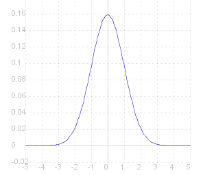
One of the most commonly met examples of a contiuous random variable is the Normal Distribution . This is actually a family of distributions with the p.g.f. differing depending on a couple of parameters. Here we give as an example the ~{standard normal distribution} whose p.g.f. is
f( ~x ) _ = _ fract{1,&sqrt.${2&pi.}} e ^{- ~x^2/2 }
The graph of which looks like this:
|
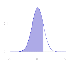
The probability that the value of the random variable is less than a given value, ~c, is given by the distribution function, F( ~c ) : F( ~c ) _ = _ fract{1,&sqrt.${2&pi.}} int{,{-&infty.},~c,} e ^{- ~x^2/2 } _ d~x This is shown (right) as the area under the graph of the p.g.f. ( where ~c = 1 ). |
 |
|
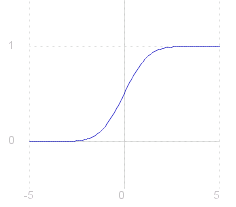
The distribution function (c.d.f.) of the normal distribution cannot be given as an explicit function, but only as an integral (above). To calculate the distribution for specific values of ~c, the student has recourse to printed statistical tables, such as Neave , or to computer packages such as the Look-up facility on this site. The graph of the distribution function for the standard normal distribution is shown (right). |
 |
Details of the normal and other continuous random variables are given in Appendix 2: Continuous Distributions .
Expectation
If ~X is a random variable, and the density function f_~X exist; , then the #~{expectation} or #~{mean} of ~X is given by
E( ~X ) _ = _ int{,{-&infty.},{+&infty.},} ~t f_~X ( ~t ) d~t
Example:
For the standard normal distribution introduced above, the expectation is
E( ~X ) _ = _ fract{1,&sqrt.${2&pi.}} int{,{-&infty.},&infty.,} ~x e ^{- ~x^2/2 } _ d~x
but note that the function _ g( ~x ) _ = _ ~x e ^{- ~x^2/2 } _ is anti-symmetric about 0, i.e. _ g( -~x ) _ = _ - g( ~x ) . _ So
int{,{-&infty.},0,} ~x e ^{- ~x^2/2 } _ d~x _ = _ - int{,0,&infty.,} ~x e ^{- ~x^2/2 } _ d~x
and
int{,{-&infty.},&infty.,} ~x e ^{- ~x^2/2 } _ d~x _ = _ int{,{-&infty.},0,} ~x e ^{- ~x^2/2 } _ d~x _ + _ int{,0,&infty.,} ~x e ^{- ~x^2/2 } _ d~x _ = _ 0
So we have that the mean of a variable with the standard normal distribution is zero.
Variance
As for discrete random variables , if ~X is a random variable and ~X ^2 has finite expectation, then we define the #~{variance}:
var( ~X ) _ = _ &sigma.^2 _ = _ E( [ ~X - E( ~X ) ]^2 ) _ = _ E( ~X ^2 ) - E( ~X )^2
Actual calculations can be done when we have looked at the distribution of the square of a random variable .
Source for the graphs shown on this page can be viewed by going to the diagram capture page .