Multiple Integration

Double Integrals

If _ ~f ( ~x ) _ is a function of the single variable _ ~x , _ defined on the interval _ ~I . _ If the interval is divided into a number of subintervals, we define the integral of _ ~f _ over this interval as:

int{ _ ~f ( ~x ),~I,,d~x} _ = _ lim{,sup_~i ( &delta.~x_~i ) -> 0} sum{ _ ~f ( ~x_~i ) &delta.~x_~i,~i,}

where ~x_~i is a point in the ~i^{th} interval and &delta.~x_~i its length. The limit is taken as the supremum over all such subdivisions of the length of all the intervals tends to zero.

In a similar way, if _ ~f ( ~x , ~y ) _ is a function of two variables defined over the area ~A of the ~x~y-plane, and if ~A is divided up into a number of sub-areas then the integral of ~f ( ~x , ~y ) over ~A is defined

dblint{ _ ~f ( ~x {,} ~y ),,,~A,,d~A} _ = _ lim{,sup_{~i} ( &delta.~A_{~i} ) -> 0} rndb{ sum{ _ ~f ( (~x {,} ~y )_~i ) &delta.~A_{~i},~i,}}

where _ ( ~x , ~y )_~i _ is a point in the ~i^{th} sub-area and &delta.~A_~i its area.

 

Rectangular Coordinates

The above definition is of little use for actual evaluations. These are done by using various specific subdivisions of the ~x~y-plane:

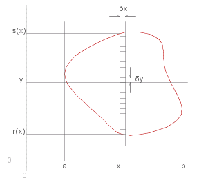
The most commons subdivison of the area is achieved by drawing a grid with equally spaced lines parallel to the ~x-axis and equally spaced lines parallel to the ~y-axis. The integral can then be calculated by taking each cell from bottom to top in a column at a time, taking the columns from left to right.

dblint{ _ ~f,,,~A,,d~A} _ ~~ _ sum{,~x = ~a,~x = ~b}rndb{ sum{ _ ~f ( ~x {,} ~y ) &delta.~x &delta.~y ,~y = ~r(~x),~y = ~s(~x)}}

which in the limit becomes:

dblint{ _ ~f,,,~A,,d~A} _ = _ int{,~a,~b,} rndb{ int{ _ ~f ( ~x {,} ~y ),~r(~x),~s(~x),d~y} } d~x

as &delta.~x -> 0 and &delta.~y -> 0 .

It is important to notice that the inner term, _ ~{∫}_~r^~s ~f(~x,~y) d~y, _ is a function of ~x only, i.e. ~y has been 'integrated out', and that the limits of the inner integral , ~r and ~s, are also functions of ~x, defined by the area over which the integration takes place.

For this reason, the order of integration cannot be changed without taking account of the endpoints. I.e. if instead of summing the cells column by column, we summed the cells row by row we would get

dblint{ _ ~f,,,~A,,d~A} _ = _ int{,~r,~s,} rndb{ int{ _ ~f ( ~x {,} ~y ),~a(~y),~b(~y),d~x} } d~y

note that ~r and ~s are now the absolute limits, whereas the limits for the integral with respect to ~x are dependent on ~y.

Example

Integrate the function _ ~f _ = _ 2~x^2 + ~y _ over the area between the lines _ ~y = ~x _ and _ ~y = ~x^2 , _ for _ 0 =< ~x =< 1.

Let _ ~I _ represent the integral, then

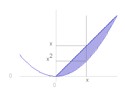
~I _ = _ int{,0,1,} rndb{ int{( 2~x&powtwo. + ~y ),~x^2,~x,d~y} } d~x

_ _ = _ int{,0,1,} script{sqrb{ 2~x&powtwo.~y + 0.5~y&powtwo. },,,~x,~x&powtwo.} d~x

_ _ = _ int{,0,1,} 2~x^3 + 0.5~x^2 - 2.5~x^4 _ d~x

_ _ = _ script{sqrb{ 0.5~x^4 + ~x^3/6 - 0.5~x^5 },,,1,0} _ = _ 1 ./ 6

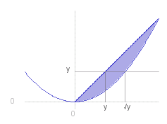
Alternatively we could have integrated over ~x first:

~I _ = _ int{,0,1,} rndb{ int{( 2~x&powtwo. + ~y ),~y,&sqrt.~y,d~x} } d~y

_ _ = _ int{,0,1,} script{sqrb{ 2~x&powthree./3 + ~y~x },,,&sqrt.~y,~y} d~x

_ _ = _ int{,0,1,} 5/3 ~y^{3/2} - 2/3 ~y^3 - ~y^2 _ d~y

_ _ = _ script{sqrb{ 2/3 ~y^{5/2} - 1/6 ~y^4 - ~y^3/3 },,,1,0} _ = _ 1 ./ 6

Polar Coordinates

Another possible subdivision is taking polar coordinates, with equally spaced spokes and equally spaced arcs dividing the area over which the integral is taken

 

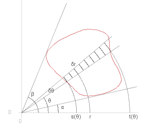
The area of the cell at ( ~r , &theta. ) is _ ~r &delta.&theta. &delta.~r , _ and the integral is given approximately by

dblint{ _ ~f,,,~A,,d~A} _ ~~ _ sum{,&theta. = &alpha.,&theta. = &beta.}rndb{ sum{ _ ~f ( ~r {,} &theta. ) ~r &delta.&theta. &delta.~r ,~r = ~s(&theta.),~r = ~t(&theta.)}}

taking the limit as &delta.&theta. -> 0 and &delta.~r -> 0:

dblint{ _ ~f,,,~A,,d~A} _ = _ int{,&alpha.,&beta.,} rndb{ int{ _ ~r ~f ( ~r {,} &theta. ),~s(&theta.),~t(&theta.),d~r} } d&theta.

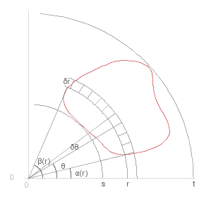
Alternatively we can sum by arc (see right) in which case the integral is given by

dblint{ _ ~f,,,~A,,d~A} _ = _ int{~r,~s,~t,} rndb{ int{ _ ~f ( ~r {,} &theta. ),&alpha.(~r),&beta.(~r),d&theta.} } d~r

Note the limits of integration, and also that we have put ~r outside the integral by &theta., though this is not necessary, it depends on the function that is being integrated.

Example

Integrate the function _ ~f _ = _ ~x _ over the quadrant defined by _ ~y^2 + ~x^2 =< ~a^2 , _ ~x >= 0 , _ ~y >= 0.

In polar coordinates this quadrant is given by _ 0 =< ~r =< ~a , _ 0 =< &theta. =< &pi./2 , _ and _ ~x _ = _ ~r cos &theta. . So the integral, ~I, is

~I _ = _ int{,0,&pi./2,} rndb{ int{( ~r&powtwo. cos &theta. ),0,~a,d~r} } d&theta.

Note that in this case the order of integration makes no difference, as the limits are independent of the other variable in both cases, due to the shape of the area of integration.

~I _ = _ int{,0,&pi./2,} script{sqrb{ 1/3 ~r^3 cos &theta. },,,~a,0 } d&theta. _ _ = _ int{,0,&pi./2,} 1/3 ~a^3 cos &theta. _ d&theta.

_ _ = _ script{sqrb{ 1/3 ~a^3 sin &theta. },,,&pi./2,0 } _ = _ ~a^3 ./ 3

The same result would have been obtained by integrating over &theta. first (this is left as an exercise). Also as an exercise, try to obtain the integral by integrating using rectanglar coordinates.

---